Phase 11. Demand cycle

The adoption fraction in our model is constant each period. Actually it changes in a complex way since the demand on our product follows the cycle of the seasons. The peak of the demand is in summer while in winter the product is in little demand. There is also a little peak in adopter activity before the New Year holiday. We want to model the demand cycle and its affect on the adoption fraction in our model.

Assume that we have experimental data how the average demand on the product changes during the year. We will use a table function to add this data to our model. Table function is a function defined in the table form. It returns tabulated values for defined argument values. If the function argument does not correspond to any of the tabulated values, table function computes a value based on the chosen interpolation.

Define the demand curve with a table function

1. Drag the  Table Function element from the  System Dynamics palette onto the Main diagram.
2. Go to the table function’s Properties and set up the function properties.
3. Name the function demand.
4. Define data for a table function in the Table Data table. Each “argument-value” pair is specified in an individual row of the table. To define pair of values, click the empty Argument cell and enter a new argument of the function. Then click the adjacent Value cell to the right and enter the function value for this argument.
   

   Define the function values: click More, then the Copy code button which appears in the top right corner of the code block.

   1	3
   2	3,6
   3	4,1
   4	6,3
   5	7,7
   6	9,6
   7	10,1
   8	9,7
   9	7,4
   10	4,8
   11	3,9
   12	6,3

   Then, click Paste from Clipboard below the table.
   The result should look like the following figure: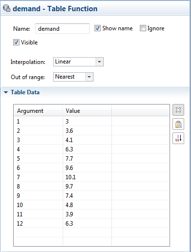

   

5. Define how the table function is interpolated. From the Interpolation drop-down list, choose Linear. The function will take a straight line between data points.
6. Define how the function behaves when the provided arguments are out-of-range. From the Out Of Range drop-down list, choose Nearest option. In the case of out-of-range arguments the function will raise an error. The function will use the nearest valid argument for out-of-range arguments.

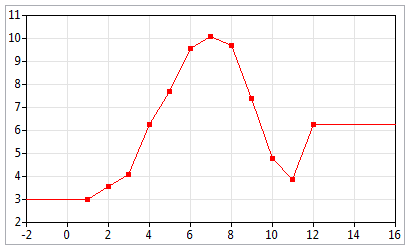
Finally you will see how the demand curve looks in the function’s preview chart on the function’s properties page:

Now we want to model how the adoption fraction depends on the current demand on the product. Therefore we will define a custom function and replace the  AdoptionFraction parameter with the dynamic variable, which value is calculated according to this function.

Define a function evaluating the adoption fraction

1. Drag the  Function element from the  Agent palette onto the Main diagram.
2. Go to the function’s Properties and name the function adoptFraction.
3. Specify that the function returns the double value. Choose the Returns value option and leave double as the return Type.
4. Open the Function body section of the Properties and enter the function expression. Type here the following string instead of existing one:
   return demand( getMonth() )/200.0;

This expression calculates the demand for the current month. Finally, to obtain the adoption fraction value, the demand value is divided by the conversion factor.

getMonth() is AnyLogic predefined function. You can use frequently used functions (sin(), time(), getDay(), etc.) in your expressions. Entering expressions, you can use code completion, where predefined functions are listed as well as variables.

Finally, we will replace the adoption fraction constant with the dynamic variable evaluating its value with the created function.

Replace AdoptionFraction parameter with a dynamic variable

1. Delete  AdoptionFraction parameter.
2. Create the AdoptionFraction dynamic variable. Set the variable’s formula to adoptFraction(). Thus, the dynamic variable’s value will be computed by our function.

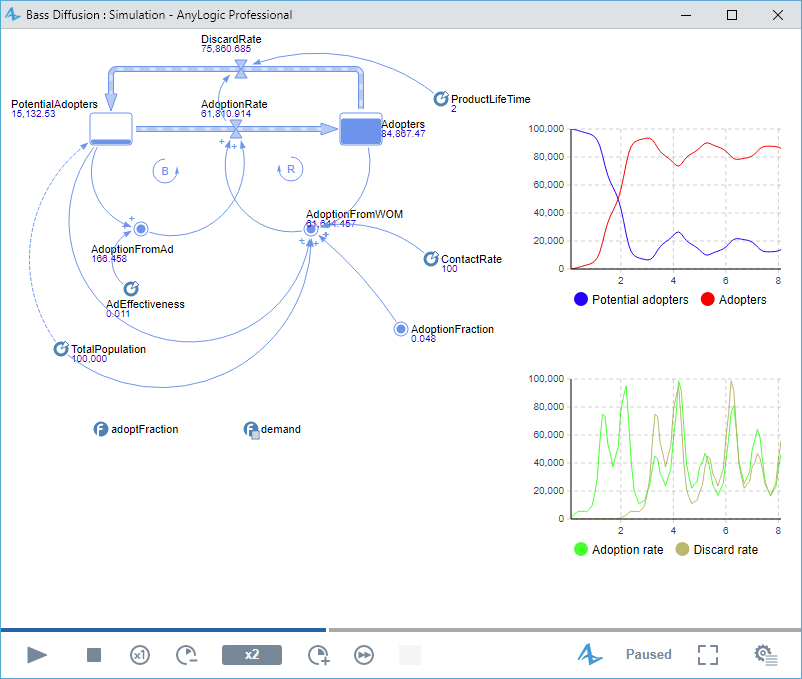
Set model to stop at time 20 (setting the stop time is described in the Phase 7) and run the model. You can see that now the behavior of a model deviates above and below an equilibrium point since the adoption rate and the discard rate oscillate.

How can we improve this article?

Send