Optimization experiment

Optimization is the process of finding the optimal combination of conditions resulting in the best possible solution. Optimization can help you find, for example, the optimal performance of a server or the best method for processing bills.

If you need to run a simulation and observe system behavior under certain conditions, as well as improve system performance by making decisions about system parameters and structure, create the optimization experiment in AnyLogic.

The optimization experiment supports two optimization engines:

• Genetic is an optimization engine based on an evolutionary algorithm, aiming to preserve the diversity of possible solutions and avoid stucking on suboptimal solutions. Instead of generating a single solution during each step, the engine generates a population of solutions, saving the best of them for the next step and so on, until the best possible solution is reached.
• OptQuest optimization engine is a proprietary tool by OptTek Systems, Inc. which provides a general-purpose, “black-box” global optimization algorithm.

For both engines, AnyLogic provides a convenient graphical user interface to set up and control the optimization — and enables exporting models with optimization experiments as standalone applications.

The optimization process consists of repetitive simulations of a model with different parameters. Using sophisticated algorithms, the optimization engine varies controllable parameters from simulation to simulation to find the optimal parameters for solving a problem.

You can control the optimization experiment with Java code.

To optimize your model

1. Create a new optimization experiment.
2. Select the optimization engine.
3. Define optimization parameters (parameters to be varied).
4. Create the experiment UI.
5. Specify the function to be minimized or maximized (the objective function).
6. Define constraints and requirements to be met (optional).
7. Specify the simulation stop condition.
8. Specify the optimization stop condition.
9. Run the optimization.

The last step of the System dynamics tutorial explains how to create and run optimization step-by-step.

To create an optimization experiment

1. In the Projects view, right-click (macOS: Ctrl + click) the model item and choose New > Experiment from the popup menu. The New Experiment dialog box is displayed.
2. Choose the Optimization option from the Experiment Type list.
3. Type the experiment name in the Name edit box.
4. Choose the top-level agent of the experiment from the Top-level agent drop-down list.
5. If you want to apply model time settings from another experiment, leave the Copy model time settings from check box selected and choose the experiment in the drop-down list to the right.
6. Click Finish.

General

Name — The name of the experiment.

Since AnyLogic generates a Java class for each experiment, please follow Java naming guidelines and start the name with an uppercase letter.

Ignore — If selected, the experiment is excluded from the model.

Top-level agent — Using the drop-down list, choose the top-level agent type for the experiment. The agent of this type will play a role of a root for the hierarchical tree of agents in your model.

Optimization engine — The optimization engine used by the experiment: OptQuest or Genetic.

Objective — The objective function you want to minimize or maximize. The top-level agent is accessible here as root.

Number of iterations — If selected, optimization will be stopped, if the maximum number of simulations, specified in the field to the right, is exceeded.

The Genetic optimization engine does not support the Infinite number of iterations.

Automatic stop — If selected, optimization will be stopped, if the value of the objective function stops improving significantly (this option is named optimization autostop).
If the Genetic optimization engine is used, the Automatic stop property becomes invisible: it is always on due to the technical specifics.

Maximum available memory — The maximum size of the Java heap allocated for the model.

Create default UI — The button creates the default UI for the experiment.

Click this button only after you completely set up the optimization parameters in the Parameters section and the experiment's objective function. It will delete the currently existing experiment UI and will create the new one corresponding to the current experiment's settings.

Parameters

Parameters — Defines the set of optimization parameters (also known as decision variables). The table lists all the parameters of the top-level agent.
To make a parameter a decision variable, click in the Type field and choose the type of the optimization parameter other than fixed.
Depending on the type of the parameter, the list of possible values may vary: discrete for int, continuous and discrete for double, and so on.
Specify the range for the parameter. Enter the parameter’s lower bound in the Min field and the parameter’s upper bound in the Max field. For discrete parameters, specify the increment value in the Step field.

Model time

Stop — Defines whether the model will Stop at specified time, Stop at specified date, or it will Never stop. In the first two cases, the stop time is specified using the Stop time/Stop date controls.

Start time — The initial time for the simulation time horizon.

Start date — The initial calendar date for the simulation time horizon.

Stop time — [Enabled if Stop is set to Stop at specified time] The final time for the simulation time horizon (the number of model time units for the model to run before it will be stopped).

Stop date — [Enabled if Stop is set to Stop at specified date] The initial calendar date for the simulation time horizon.

Additional optimization stop conditions — Here you can define any number of additional optimization stop conditions. When any of these conditions will be evaluated to true, optimization will be stopped. A condition can include checks of dataset mean confidence, variable values, and so on. The top-level agent of the experiment can be accessed here as root, so if you want, for example, to stop the optimization when the variable var of the experiment’s top-level agent steps over the threshold, type root.var > 11.
To make the condition active, select the checkbox in the corresponding row of the table.

Constraints

Defines the constraints — additional restrictions imposed on the optimization parameters.

Constraints on simulation parameters (are tested before a simulation run) — The table that defines the optimization constraints. A constraint is a condition defined upon optimization parameters. It defines a range for an optimization parameter. Each time the optimization engine generates a new set of values for the optimization parameters, it creates feasible solutions, satisfying this constraint; thus the space for searching is reduced, and the optimization is performed faster.
A constraint is a well-formed arithmetic expression describing a relationship between the optimization parameters. It always defines a limitation by specifying a lower or an upper bound, for example, parameter1 >= 10. Constraints are calculated before the model run and instantiation of the top-level agent, so they cannot involve any of the top-level agent’s contents.
Each constraint is defined in an individual row of the table and can be disabled by deselecting the corresponding checkbox in the first column.

Requirements

Defines the requirements — additional restrictions imposed on the solutions found by the optimization engine.

Requirements (are tested after a simulation run to determine whether the solution is feasible) — The table defining the optimization requirements. A requirement is an additional restriction imposed on the solution found by the optimization engine. Requirements are checked at the end of each simulation, and if they are not met, the current parameter values are rejected.
A requirement can also be a restriction on a response that requires its value to fall within a specified range. It may contain any variables, parameters, functions, etc. of the experiment’s top-level agent accessible in the expression field as root.
Each requirement is defined in an individual row of the table and can be disabled by deselecting the corresponding checkbox in the first column.

Randomness

Random number generator — Here you specify, whether you want to initialize a random number generator for this model randomly or with some fixed seed. This makes sense for stochastic models. Stochastic models require a random seed value for the pseudorandom number generator. In this case model runs cannot be reproduced since the model random number generator is initialized with different values for each model run. Specifying the fixed seed value, you initialize the model random number generator with the same value for each model run, thus the model runs are reproducible. Moreover, here you can substitute AnyLogic default RNG with your own RNG.

• Random seed (unique simulation runs) — If selected, the seed value of the random number generator is random. In this case, the random number generator is initialized with the same value for each model run, and the model runs are unique (non-reproducible).
• Fixed seed (reproducible simulation runs) — If selected, the seed value of the random number generator is fixed (specify it in the Seed value field). In this case, the random number generator is initialized with the same value for each model run, and the model runs are reproducible.
• Custom generator (subclass of Random) — If for any reason you are not satisfied with the quality of the default random number generator Random, you can substitute it with your own one. Just prepare your custom RNG (it should be a subclass of the Java class Random, for example, MyRandom), choose this particular option, and type the expression returning an instance of your RNG in the field on the right, for example, new MyRandom() or new MyRandom( 1234 ).
  You can find more information in Custom number generator.

Replications

Use replications — if selected, the optimization engine will run several replications per simulation. You need this when your model contains stochastics. In such cases, the results of the simulation runs are unique and the values of the optimized function which are obtained for the simulation runs executed with the same values of optimization parameters most likely differ from each other. We cannot execute only one simulation run, accept its results as the current iteration result, and proceed with optimization by checking other parameter values. To obtain reliable representative data, we need to execute several runs (called “replications” here) for a single set of parameter values and accept the mean of all replications results as the values of the objective.

Fixed number of replications — if selected, a fixed number of replications will be run per each simulation.

• Replications per iteration — [enabled if Fixed number of replications is set] The fixed number of replications, which will be run per each simulation.

Varying number of replications (stop replications after minimum replications, when confidence level is reached) — If selected, a varying number of replications will be run per each simulation. When running a varying number of replications, you will specify the minimum and the maximum number of replications to be run. The OptQuest engine will always run the minimum number of replications for a solution. OptQuest then determines if more replications are needed. The OptQuest engine stops evaluating a solution when one of the following occurs:

• The true objective value is within a given percentage of the mean of the replications to date.
• The current replication objective value is not converging.
• The maximum number of replications has been run.

The Genetic optimization engine does not support Varying number of replications.

For this property, the following options are available:

• Minimum replications — [enabled if Varying number of replications is set] The minimum number of replications the OptQuest engine will always run per one simulation.
• Maximum replications — [enabled if Varying number of replications is set] The maximum number of replications the OptQuest engine can run per one simulation.
• Confidence level — [enabled if Varying number of replications is set] — The confidence level to be evaluated for the objective. The confidence level displays the probability of a random result placing within the confidence interval. You can look at it as the sample’s accuracy. As a rule, 95% is used, but in cases where high accuracy is not needed, you can use 90% and even 85%. Vice versa, the larger is the sample, the higher accuracy can be established. The confidence interval should be seen as a measure of inaccuracy. It defines the reach of the distribution curve on both sides of the selected point where the results may fall.
• Error percent — [enabled if Varying number of replications is set] — A value from 0 to 1, which defines the size of the confidence interval, that should satisfy us as the condition to stop executing additional replications for the current iteration. The interval is calculated as (current_mean_value - current-mean-value * error percent, current mean value + current mean value * error percent).

Window

Window properties define the appearance of the model window that will be shown when the user starts the experiment.

The size of the experiment window is defined using the model frame and applies to all experiments and agent types of the model.

Title — The title of the model window.

Enable zoom and panning — If selected, the user will be allowed to pan and zoom the model window.

Enable developer panel — Select/clear the checkbox to enable/disable the developer panel in the model window.

Show developer panel on start — [Enabled only if the Enable developer panel checkbox is selected] If selected, the developer panel will be shown by default in the model window every time you run the experiment.

Java actions

Initial experiment setup — The code that is executed on the experiment setup.

Before each experiment run — The code that is executed before each simulation run.

Before simulation run — The code that is executed before the simulation run. This code is run on the setup of the model. At this moment the top-level agent of the model is already created, but the model is not started yet. You may perform here some actions with elements of the top-level agent, e.g assign actual parameter values here.

After simulation run — The code that is executed after the simulation run. This code is executed when the simulation engine finishes the model execution (the Engine.finished() function is called). This code is not executed when you stop your model by clicking the Terminate execution button.

After iteration — The code that is executed after the iteration run.

After experiment — The code that is executed after the experiment run.

Advanced Java

Imports section — import statements needed for correct compilation of the experiment class’ code. When Java code is generated, these statements are inserted before the definition of the Java class.

Additional class code — Arbitrary member variables, nested classes, constants, and methods are defined here. This code will be inserted into the experiment class definition. You can access these class data members anywhere within this experiment.

Java machine arguments — Specify here the Java machine arguments you want to apply on launching your model. You can find detailed information on possible arguments at Java Sun Microsystems website: http://java.sun.com/j2se/1.5.0/docs/tooldocs/windows/java.html.

Command-line arguments — Here you can specify command-line arguments you want to pass to your model. You can get the values of passed argument values using the String[] getCommandLineArguments() method from any code field of your choice. The only exception is the values of static variables since these are initialized before the experiment class itself.

Advanced

Allow parallel evaluations — If the option is selected and the processor has several cores, AnyLogic will run several experiment iterations in parallel on different processor cores. Thereby performance is multiply increased and the experiment is performed significantly quicker. This feature is made controllable because in some rare cases, parallel evaluations may affect the optimizer strategy so that more iterations are required to find the optimal solution.
Do not use static variables, collections, table functions, and custom distributions (check that their advanced option Static is deselected), if you turn on parallel evaluations here.

Load top-level agent from snapshot — If selected, the experiment will load the model state from the snapshot file specified in the control to the right. The experiment will be started from the time when the model state was saved.

The goal of the optimization process is to find the parameter values that result in a maximum or minimum of a function called the objective function.

An objective function is a mathematical expression describing the relationship of the optimization parameters or the result of an operation (such as simulation) that uses the optimization parameters as inputs. The optimization objective is the objective function plus the optimization criterion. The latter determines whether the goal of the optimization is to minimize or maximize the value of the objective function.

To define the objective function

1. In the Projects view, click the optimization experiment.
2. In the Properties view, specify the objective function in the Objective edit box. You can enter any Java expression as an objective function. Since the expression is considered to be in the context of the top-level agent, it can access the variables and parameters of the top-level agent. The top-level agent is accessible here as root. If your algorithm is rather sophisticated, you can define a function in the top-level agent (for example, Main) and place the function call in the Objective edit box, like this: root.totalCost().
3. Define the optimization criterion. Choose Minimize/Maximize option to minimize/maximize your objective function.

The optimization engine obtains a sample of the objective function at the end of each simulation. The engine analyzes a sample (a batch of samples if the Genetic optimization engine is used), modifies optimization parameters according to its optimization algorithm, and starts a new simulation.

Therefore, optimization is an iterative process where:

• The optimization engine calculates possible solutions for the parameters
• The objective function and constraints are evaluated using the suggested solutions
• The results are analyzed by the optimization engine, and a new set of possible solutions is calculated

An optimization parameter (or a decision variable, in the terms of optimization) is a model parameter to be optimized. For example, the number of nurses to employ during the morning shift in an emergency room may be an optimization parameter in a model of a hospital. The optimization engine searches through possible values of optimization parameters to find optimal parameters. It is possible to have more than one optimization parameter.

Only a parameter of the top-level agent of the optimization experiment can be an optimization parameter, so you must have at least one parameter in this agent. If you need to optimize the parameters of embedded agents, use parameter propagation.

The dimension of the search area depends on the number of optimization parameters. Each new parameter expands the search area, thus slowing down the optimization. If you have N optimization parameters, their ranges form the N-dimensional square search area. Obviously, that area must be wide enough to contain the optimal point. However, the wider the range is, the more time is needed to find the optimum in the search area. On the other hand, if the OptQuest optimization engine is used, suggested parameter values located near the optimal value can shorten the time it takes to find the optimal solution.

During the optimization process, the parameter’s value is changed in accordance with its type within an interval specified by lower and upper bounds. There are the following types of optimization parameters:

• Boolean parameter
• Continuous parameter
• Discrete parameter

A boolean parameter can have true or false as its value.

A continuous parameter can take any value from the interval. The parameter precision determines the minimal value continuous parameters can change.

A discrete parameter is represented by a finite set of decisions with essential direction: the parameter influences the objective like a numeric parameter but can take values from the specified set only. It begins at a lower bound and increments by a step size up to an upper bound.

Sometimes the range and step are exactly defined by the problem, but generally, you will have to choose them. If you specify the step for the parameter, only the discrete points will be involved in the optimization, so it will be impossible to determine the optimal parameter value more precisely than defined by the step. So, if you are not sure what the step should be, choose the Continuous rather than the Discrete parameter type.

Optimization parameters are defined in the Parameters section of the optimization experiment properties. The table already lists all parameters of the top-level agent. By default, all of them are fixed, that is, they are not varied by the optimization process.

To make a parameter a decision variable

1. Select the optimization experiment in the Projects view.
2. On the Parameters section of the Properties view, go to the row of the Parameters table containing the parameter you want to make a decision variable.
3. Click the Type field and choose the type of the optimization parameter. Depending on the type of parameter, the list of possible values may vary.
   If you leave the fixed value, the parameter will not be considered as a decision variable, and the optimization engine will use its default value for all experiment’s iterations.
   • For the boolean parameter, choose boolean to make it an optimization parameter. The optimization engine will take either true or false as the parameter value.
   • For the int parameter, choose discrete to make it an optimization parameter. The parameter will take values only from the limited set of values within the specified value range.
     Example: Min: 0, Max: 4, Step: 2. Possible values: 0, 2, 4.
   • For the double, or unit parameter (for example, Time, Rate, and so on), choose one of the following options:
     • continuous — The most popular option. The parameter can take any values from the specified range.
     • discrete — The parameter will take only values from the limited set of values within the specified value range only.
       Example: Min: 0, Max: 1, Step: 0.5. Possible values: 0, 0.5, 1.
4. Specify the range for the parameter. Enter the parameter’s lower bound in the Min field and the parameter’s upper bound in the Max field.
5. For discrete parameters, specify the parameter step in the Step field.
6. If you use the OptQuest optimization engine, suggest the initial value for the parameter in the Suggested field. Initially, the value is set to the parameter’s default value, but you can enter any other value here.
   The Genetic optimization engine does not support suggested values.

You can use the following functions to control the optimization experiment, retrieve the data on its execution status and use it as a framework for creating custom experiment UI.

Controlling execution

Function	Description
void run()	Starts the experiment execution from the current state. If the model does not exist yet, the function resets the experiment, then creates and starts the model.
void pause()	Pauses the experiment execution.
void step()	Performs one step of experiment execution. If the model does not exist yet, the function resets the experiment, then creates and starts the model.
void stop()	Terminates the experiment execution.
void close()	This function returns immediately and performs the following actions in a separate thread: Stops experiment if it is not stopped, Destroys the model, Closes the experiment window (only if the model is started in the application mode).
Experiment.State getState()	Returns the current state of the experiment: IDLE, PAUSED, RUNNING, FINISHED, ERROR, or PLEASE_WAIT.
double getRunTimeSeconds()	Returns the duration of the experiment execution in seconds, excluding pause times.
int getRunCount()	Returns the number of the current simulation run, i.e., the number of times the model was destroyed.
double getProgress()	Returns the progress of the experiment: a number between 0 and 1 corresponding to the currently completed part of the experiment (a proportion of completed iterations of the total number of iterations), or -1 if the progress cannot be calculated.
int getParallelEvaluatorsCount()	Returns the number of parallel evaluators used in this experiment. On multicore / multiprocessor systems that allow parallel execution, this number may be greater than 1.

Objective

Function	Description
double getCurrentObjectiveValue()	Returns the value of the objective function for the current solution.
double getBestObjectiveValue()	Returns the value of the objective function for the optimal currently found solution. The solution may be infeasible. To check the solution feasibility, call the isBestSolutionFeasible() function.
double getSelectedNthBestObjectiveValue()	Returns the objective value for the Nth best solution identified by the function selectNthBestSolution(int). The Genetic optimization engine does not support this function.

Solution

Function	Description
boolean isBestSolutionFeasible()	Returns true if the optimal solution satisfies all constraints and requirements; returns false otherwise.
boolean isCurrentSolutionBest()	Returns true if the solution is currently the optimal one; returns false otherwise.
boolean isCurrentSolutionFeasible()	Returns true if the current solution satisfies all constraints and requirements; returns false otherwise.
boolean isSelectedNthBestSolutionFeasible()	Returns true if the Nth best solution satisfies all constraints and requirements; returns false otherwise. The Genetic optimization engine does not support this function.
void selectNthBestSolution (int bestSolutionIndex)	This function locates the Nth best solution and sets up the data for subsequent function calls that retrieve specific pieces of information (for example, for the getSelectedNthBestObjectiveValue() and getSelectedNthBestParamValue(IVariable) functions). bestSolutionIndex — the index of the optimal solution (passing 1 will locate the optimal solution, 2 — the second optimal, etc.). The Genetic optimization engine does not support this function.

Optimization parameters

Function	Description
double getCurrentParamValue(IVariable optimizationParameterVariable)	Returns the value of the given optimization parameter variable for the current solution.
double getBestParamValue(IVariable optimizationParameterVariable)	Returns the value of the given optimization parameter variable for the optimal currently found solution. The solution may be infeasible. To check the solution feasibility, call the isBestSolutionFeasible() function.
double getSelectedNthBestParamValue(IVariable optimizationParameterVariable)	Returns the value of the variable for the Nth best solution identified by calling the selectNthBestSolution(int) function. The Genetic optimization engine does not support this function.

Iterations

Function	Description
int getCurrentIteration()	Returns the current value of the iteration counter.
int getBestIteration()	Returns the iteration that resulted in the optimal currently found solution. The solution may be infeasible. To check the solution feasibility, call the isBestSolutionFeasible() function.
int getMaximumIterations()	Returns the total number of iterations.
int getNumberOfCompletedIterations()	Returns the number of completed iterations.
int getSelectedNthBestIteration()	Returns the iteration number for the Nth best solution identified by the selectNthBestSolution(int) function. The Genetic optimization engine does not support this function.

Replications

Before calling the optimization experiment functions you may need to ensure that replications are used (call the isUseReplications() function).

Function	Description
boolean isUseReplications()	Returns true if the experiment uses replications; returns false otherwise.
int getCurrentReplication()	Returns the number of replications run so far for the currently evaluated solution.
int getBestReplicationsNumber()	Returns the number of replications that were run to get the optimal solution. The solution may be infeasible. To check the solution feasibility, call the isBestSolutionFeasible() function.
int getSelectedNthBestReplicationsNumber()	Returns the number of replications for the Nth best solution identified by the selectNthBestSolution(int) function. The Genetic optimization engine does not support this function.

Accessing the model

Function	Description
Engine getEngine()	Returns the engine executing the model. To access the model’s top-level agent (typically, Main), call getEngine().getRoot();.
IExperimentHost getExperimentHost()	Returns the experiment host object of the model, or some dummy object without functionality if the host object does not exist.

Restoring the model state from the snapshot

Function	Description
void setLoadRootFromSnapshot(String snapshotFileName)	Tells the simulation experiment to load the top-level agent from the AnyLogic snapshot file. This function is only available in AnyLogic Professional. snapshotFileName — the name of the AnyLogic snapshot file, for example: "C:\My Model.als"
boolean isLoadRootFromSnapshot()	Returns true if the experiment is configured to start the simulation from the state loaded from the snapshot file; returns false otherwise.
String getSnapshotFileName()	Returns the name of the snapshot file, from which this experiment is configured to start the simulation.

Error handling

Function	Description
RuntimeException error(Throwable cause, String errorText)	Signals an error during the model run by throwing a RuntimeException with errorText preceded by the agent’s full name. This function never returns, it throws a runtime exception by itself. The return type is defined for the cases when you would like to use the following call form: throw error("my message"); cause — the cause (which will be saved for a more detailed message), may be null. errorText — the text describing the error that will be displayed.
RuntimeException errorInModel(Throwable cause, String errorText)	Signals a model logic error during the model run by throwing a ModelException with specified error text preceded by the agent’s full name. This function never returns, it throws a runtime exception by itself. The return type is defined for the cases when you would like to use the following call form: throw errorInModel("my message"); This function differs from error() in the way of displaying an error message: model logic errors are “softer” than other errors, they use to happen in the models and signal to the model developer that the model might need some parameter adjustments. Examples: “agent was unable to leave flowchart block because subsequent block was busy”, “insufficient capacity of pallet rack”, etc. cause — the cause (which will be saved for a more detailed message), may be null. errorText — the text describing the error that will be displayed.
void onError (Throwable error)	This function may be overridden to perform custom handling of the errors that occurred during the model execution (i.e., errors in the action code of events, dynamic events, transitions, entry/exit codes of states, formulas, etc.). By default, this function does nothing as its definition is empty. To override it, you can add a function to the experiment, name it onError and define a single argument of the java.lang.Throwable for it. error — an error that has occurred during event execution.
void onError (Throwable error, Agent root)	Similar to onError(Throwable error) function except that it provides one more argument to access the top-level (root) agent of the model. error — an error that has occurred during event execution. root — the top-level (root) agent of the model. Useful for experiments with multiple runs executed in parallel. May be null in some cases (e.g. on errors during top-level agent creation).

Command-line arguments

Function	Description
String[] getCommandLineArguments()	Returns an array of command-line arguments passed to this experiment on model start. Never returns null: if no arguments are passed, an empty array is returned. Cannot be called from within a value of a static variable: these are initialized before the experiment class itself.

AnyLogic supports constraints and requirements — additional restrictions imposed on the optimization parameters and solutions found by the optimization engine.

A constraint is a more complex condition defined upon optimization parameters, which is tested each time the optimization engine generates a new set of values. It is used in cases when the value of a decision variable must be described more precisely than simply a range in Parameters.

Usually, a constraint is a well-formed arithmetic expression describing a relationship between the optimization parameters.

parameterA + parameterB + 2 * parameterC = 10
parameterC - parameterA * parameterB >= 300

• A linear constraint defines a linear relationship among variables. OptQuest is able to test a value against a linear constraint and determine if this value violates the constraint without running the model.
• A non-linear constraint is applicable in the situation the expression itself is non-linear or contains an output of the simulation (that is, the variable value is controlled by a user). OptQuest requires the model run to test the non-linear constraints.

To define a constraint

1. Select the optimization experiment by clicking on it in the Projects view.
2. In the Constraints section of the Properties view, click the button to the right of the table Constraints on simulation parameters (are tested before a simulation run).
3. Specify the constraint in the Expression, Type, and Bound cells of the row.
4. Select the check box in the Enabled column. Otherwise, the constraint is eliminated from the optimization process and does not affect its results.

A requirement is an additional restriction imposed on the solution found by the optimization engine. Requirements are checked at the end of each simulation, and if they are not met, the parameters used are rejected. Otherwise, the parameters are accepted.

This means that if all variables meet their constraints at the end of the simulation, the corresponding set of parameter values is considered feasible, and the result of the simulation is accepted by the optimization engine. Otherwise, parameter values are considered infeasible, and the result is rejected.

A requirement can also be a restriction on a response that requires its value to fall within a specified range. Constraint may contain any variables of the agent, the model time symbol t, any arithmetic operations, and method calls, such as, for example, sin(), cos(), sqrt(), and so on, or calls to your own methods.

0 <= 2 * root.variable - root.statistics.max() <= 500
sqrt(variableC) >= 49

To define a requirement

1. Select the optimization experiment by clicking it in the Projects view.
2. In the Requirements section of the Properties view, click the button to the right of the table Requirements (are tested after a simulation run to determine whether the solution is feasible).
3. Specify the requirement in the Expression, Type, and Bound cells of the row. In the Expression field, the top-level agent is available as root.
4. Select the check box in the Enabled column. Otherwise, the requirement is eliminated from the optimization process and does not affect its results.

A feasible solution is one that satisfies all constraints and requirements. The optimization engine makes finding a feasible solution its highest priority.

The fact that a particular solution may be infeasible does not imply that the problem itself is infeasible. However, infeasible problems do exist. Here is an example:

parameterA + parameterB <= 4

parameterA + parameterB >= 5

Clearly, there is no combination that will satisfy both of these constraints.

If a model is constraint-feasible, the optimization engine will always find a feasible solution and search for the optimal solution (that is, the best solution that satisfies all constraints).

If the optimization engine cannot find any feasible solutions, you should check the constraints for feasibility and fix the inconsistencies of the relationships modeled by the constraints.

To enable optimization, you must ensure that each simulation ends. By default, a simulation never ends; therefore the optimization engine gets no samples of the objective function. To ensure that each simulation ends, you must specify a simulation stop condition. The most common and simple simulation stop condition is stopping at the specified model time.

In general, a simulation stop condition should be specified in such a way that the value of the objective function is significant when the simulation stops. The model should be stable, transient processes should be finished, and statistics should be representative.

Optimization can stop under two circumstances: the maximum number of simulations is exceeded or the value of the objective function stops improving significantly. The latter is also known as automatic stop. You can use any of these conditions to stop an optimization. If more than one condition is specified, optimization stops when the first condition is satisfied.

Set up these settings of an optimization process on the General properties page of the optimization experiment.

You can also specify additional stop conditions in the corresponding property in the Model time section of the optimization experiment’s properties. When any of these conditions will be evaluated to true, optimization will be stopped.

To stop optimization after the specified number of iterations

1. Select the optimization experiment by clicking on it in the Projects view.
2. Go to the Properties view.
3. Specify the number of iterations in the Number of iterations edit box. The optimization stops when this number is exceeded.

To switch optimization autostop on

1. Select the optimization experiment by clicking on it in the Projects view.
2. Go to the Properties view.
3. Select the Automatic Stop check box.

Just like the simulation experiment, the optimization experiment has its own presentation that is drawn on the graphical editor diagram. By default, the diagram is empty. However, AnyLogic offers the ability to create some default UI for the experiments. We advise you to start with creating the default UI and then adjust it somehow to satisfy your requirements.

To create the default optimization UI

1. Select the optimization experiment in the Projects view.
2. Go to the Properties view.
3. Click the Create default UI button. This creates the default UI for the optimization experiment as shown in the figure below.

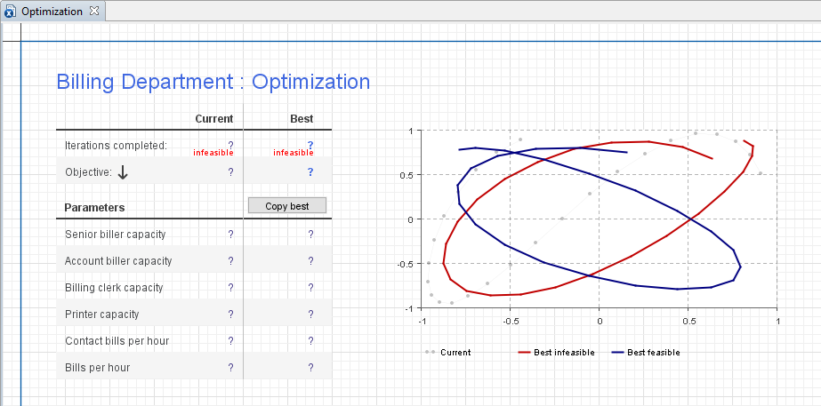   The default UI created for the optimization experiment

The default UI consists of a number of controls displaying all the necessary information regarding the current status of the optimization.

The table at the left displays all necessary information about the optimization process. The values in the column Current show the user the number of the current Iteration, Parameter values used, and the corresponding Objective found to this moment. The values in the column Best form the best solution found up to the current time. Once optimization has finished, this solution is considered to be optimal. The best value of the objective function corresponds to this optimal solution. You can copy it to the clipboard using the Copy button below.

The chart to the right visually illustrates the optimization process. The X-axis represents simulations, and the Y-axis represents Current Objective, Best Feasible Objective, and Best Infeasible Objective found for each simulation.

The optimization experiment is run by clicking the Run button situated on the control panel of the model window.

After you set up the optimization, you are ready to run it. This involves the following steps:

• Start the optimization
• Observe the status
• Determine the best solution
• (Optionally) Copy the best solution to the simulation experiment to simulate this model with optimal parameters for some time and observe its behavior

To run an optimization experiment

1. In the Projects view, right-click (macOS: Ctrl + click) your optimization experiment and choose  Run from the context menu.
2. Alternatively, choose Model > Run from the main menu, or click the arrow to the right of the  Run toolbar button and choose the experiment you want to run from the drop-down list.
3. This opens the model window, displaying the experiment’s UI. If you have created the default UI for the experiment, start the optimization by clicking the  Run button in the control panel at the bottom of the model window. The optimization process will be started.

When you have finished finding the optimal solution, you may copy it to the simulation experiment of your model. Then you will be able to simulate this model with optimal parameters.

To copy the found optimal parameters to the simulation experiment

1. When you have finished finding the optimal solution, copy the values of parameters corresponding to the best solution, to the clipboard, by clicking the copy button in the model window.
2. Paste the optimal parameter values into the simulation experiment by opening the General property page of this simulation experiment and clicking the Paste from Clipboard button at the bottom.

If your model is stochastic, the results of the single model run may not be representative; thus, you may consider to run a fixed number of replications per simulation or, with OptQuest, a varying number of replications per simulation.

When running an OptQuest experiment varying number of replications, you will specify the minimum and maximum number of replications to be run. The engine will always run the minimum number of replications for a solution. OptQuest is then able to determine if more replications are needed. The engine stops evaluating a solution when one of the following occurs:

• The true objective value is within a given percentage of the mean of the replications to date.
• The current replication objective value is not converging.
• The maximum number of replications has been run.

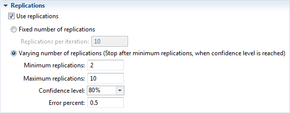Optimization experiment’s properties view. Replications section

To schedule a fixed number of replications

1. In the Projects view, select the optimization experiment.
2. In the Replications section of the Properties view, select the Use Replications check box.
3. Choose the Fixed number of replications option.
4. Specify the number of Replications per iteration in the edit box.

To schedule a varying number of replications

1. In the Projects view, select the optimization experiment.
2. In the Replications section of the Properties view, select the Use Replications check box.
3. Choose the Varying number of replications (Stop replications after minimum replications, when confidence level is reached) option.
4. Specify the minimum number of replications in the Minimum replications edit box.
5. Specify the maximum number of replications in the Maximum replications edit box.
6. Define the Confidence level to be evaluated for the objective.
7. Specify the percent of objective for which the confidence level is determined in the Error percent field.

Here are some tips you may find helpful:

• Debug your model before starting the optimization. If your model cannot run properly under some values of optimization parameters, you can restrict the search space using ranges. Otherwise, be aware of the possible incorrect model operation.
• If the optimization engine finds all solutions to be infeasible, this indicates that there is no solution in the parameter space satisfying all the constraints. Possible reasons for this are:
  • The constraints are inconsistent. Check for conflicting constraints, such as x>25, x<24. If variables appearing in the constraints are calculated using some formulas inside the model, inconsistency can be in those formulas.
  • The ranges of the optimization parameters conflict with the constraints.

If you find optimization performance unsatisfactory, consider the following recommendations.

Find an optimal solution faster

• Adjust the optimization engine settings for your problem. Fine-tuning these settings can increase optimization performance (for more information, please consult AnyLogic Class Reference):
  • Suggest initial values for optimization parameters as close to the optimal value as possible
  • Reduce the search space by specifying ranges for optimization parameters
  • Exclude parameters that do not influence the objective function
  • Avoid using constraints. First, optimize your model without constraints; then check the optimal solution for constraints. If some constraints are not satisfied, start optimizing with constraints.
• Solve the optimization problem interactively and iteratively:
  • Initially, use a rough approximation of the problem: wide ranges, big steps, and low precisions.
  • Run the optimization until the best-found value starts changing slowly.
  • Set up the optimization more precisely. Reduce ranges and steps of optimization parameters. Start with optimization parameter values obtained in the previous step.
  • Run the optimization until the best-found value starts changing slowly. If you are satisfied with the results, stop the optimization. Otherwise, return to the previous step.

In general, the optimization process may be very time-consuming, especially if there are multiple parameters. If nothing from the list above helps improve performance, try using a more powerful workstation or schedule more time for optimization.

How can we improve this article?

Send