Phase 10. Replacement purchases

The model we have created does not capture situations where the product is consumed, discarded, or upgraded, all of which lead to repeat purchases. We will model repeat purchase behavior by assuming that adopters move back into the population of potential adopters when their first unit is discarded or consumed.

First, we will define a constant representing the average lifetime of product.

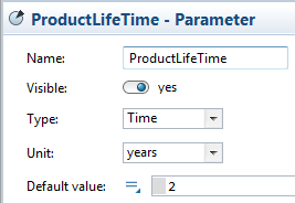
Create the ProductLifeTime constant

1. Assume that the average duration of active use of our product is 2 years. Type 2 as the Default value.

   

People move back from the adopter population to the pool of potential adopters when the product they have purchased is discarded or consumed. So, the discard flow is nothing else but the adoption flow delayed on the average lifetime of the product.

Create the discard flow from Adopters to PotentialAdopters

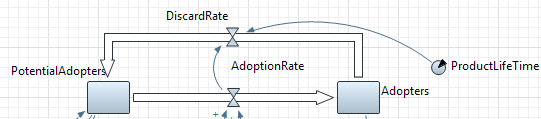
1. Now we want to add a flow going from  Adopters to  PotentialAdopters. But if we will draw it with a straight arrow, it will overlap  AdoptionRate flow on the diagram. That’s why we need to create a flow of a custom shape, like shown in the figure given below.
2. To draw a flow of a custom shape, double-click the element in the  System Dynamics palette so that its icon turns into .
3. Right after that, go to the graphical editor and click the stock where the flow flows out (  Adopters).
4. Then click in the intermediate salient points.
5. Finally, click the  PotentialAdopters stock. New flow from  Adopters to  PotentialAdopters is added.
6. Change the name of the flow to DiscardRate.

   

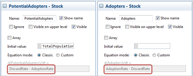
7. You can see that stock formulas have changed as well:

   

8. Set the following formula for the flow variable: delay(AdoptionRate, ProductLifeTime)

   

   The delay() function implements the time delay and has the following notation: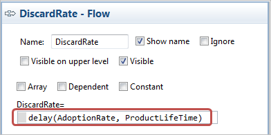
   delay(<variable>, <delay value>, <initial value>)
   In our case, the function reproduces  AdoptionRate delayed on the  ProductLifeTime value. The discard rate is null until the time of use of the first purchased products elapses.

Set DiscardRate to be displayed by the lower time plot

1. Just add DiscardRate as one more data item to be displayed by this plot (adding items onto plots is described in the previous phase).
2. Specify Discard rate as the title of this data item.

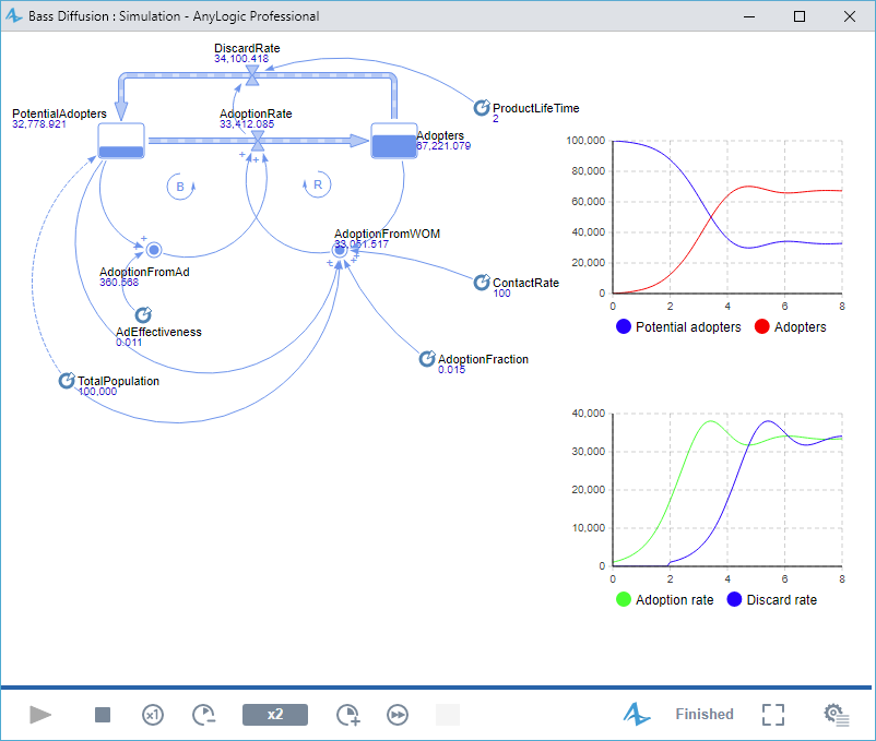
Now we have finished modeling the product replacement purchases. You may check how the delay() function works. Run the model and view plots for  AdoptionRate and  DiscardRate. You can see that rate curves look exactly how we expected — the discard rate is actually the adoption rate delayed by 2 years — the lifetime of the product.

Observe the population dynamics using the chart. Now, instead of falling to zero, the potential adopter population is constantly replenished as adopters discard the product and re-enter the market. The adoption rate rises, peaks, and falls to a rate that depends on the average life of the product and the parameters determining the adoption rate. Discards mean there is always some fraction of the population in the potential adopter pool.

If you like, you may add control group varying product lifetime, say from 0.5 to 10.

How can we improve this article?

Send