Bass diffusion model

Complexity: grade grade grade grade grade

Modeling approach: system dynamics

Features: optimization stock-and-flow diagram stock flow parameter feedback loop link table function event time plot

AnyLogic supports different modeling techniques. This document covers System Dynamics modeling approach. There are many spheres where system dynamics simulation can be successfully applied — the range of SD applications includes business, urban, social, ecological types of systems. AnyLogic allows you to create complex dynamic models using standard SD graphical notation.

This tutorial will briefly take you through the process of constructing a simulation model using AnyLogic. It is intended to introduce you to AnyLogic interface and many of its main features. We will create a simple illustrative example — the product life cycle model, used for forecasting sales of new products.

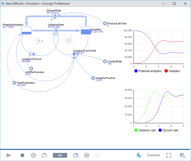
The Bass diffusion model describes a product diffusion process. Potential adopters of a product are influenced into buying the product by advertising and by word of mouth from adopters — those who have already purchased the new product. Adoption of a new product driven by word of mouth is likewise an epidemic. Potential adopters come into contact with adopters through social interactions. A fraction of these contacts results in the purchase of the new product. The advertising causes a constant fraction of the potential adopter population to adopt each time period.

The first phases will take you through the process of construction of the classic Bass diffusion model. Then we will expand our model by considering some details and introducing you to some advanced features of AnyLogic useful in creating system dynamics models. The expanded model may help you to better plan the entry strategy, target the right consumer and anticipate demand so as to have an efficient and effective promotion strategy.

• Phases 0 - 8. Creating the classic Bass Diffusion model. First, we will identify the key variables and their patterns of influence. Then, we will construct a stock-and-flow diagram consisting of stocks, flows, and dynamic variables.
• Phase 9. Adding charts. We will add two time plots to visualize the model’s behavior. One chart will show how the populations of adopters and potential adopters change over time. The other chart will display the dynamics of the adoption rate.
• Phase 10. Replacement purchases. We will consider situations where the product is consumed, discarded, or upgraded, all of which lead to repeat purchases. To model this behavior, we will assume that adopters return to the population of potential adopters once their initial unit is consumed or discarded.
• Phase 11. Demand cycle. In this phase, we will incorporate demand seasonality. To do this, we will use a table function (also known as a lookup table) to input historical monthly demand data.
• Phase 12. Promotion strategy. Since advertising plays a significant role primarily at the beginning of the diffusion process, we plan to stop advertising after a certain period. This will help us avoid unnecessary advertising expenses, as market saturation at that point is driven mainly by word-of-mouth adoption. To implement this behavior, we will add a parameter, an event, and a simple statechart with two states.
• Phase 13. Optimizing the strategy. We will conduct an optimization experiment to develop an optimal marketing plan aimed at achieving 80 per cent market saturation within 1.5 years while minimizing advertising expenditures.

How can we improve this article?

Send