Density map

AnyLogic allows you to collect statistics about the density of moving units in the simulated space and display this information in the animation as a density map. This functionality is supported for pedestrians and transporters with free space navigation.

After adding added the Density Map element, you enable the display of the density map of the specified type (pedestrian or transporter) for your simulation model.

If you have transporters and pedestrians moving on the same level and you want to track the density for both, you need to add two Density Map elements: one for each type.

You will notice that as the agents move through the simulated space, the layout is gradually painted in different colors. The color of each point in space corresponds to the current density in that particular area. The density map is constantly repainted according to the actual values: if the density changes at any point, the color changes dynamically to reflect that change. If the density is zero, the area is not painted at all. If you have transporters and pedestrians moving in the same area, the density maps will not show the total density, only a separate one for each type.

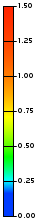
The element itself acts as the color legend for the density map. It displays the correspondence between density values and colors on the map (see the right side on the figure below).

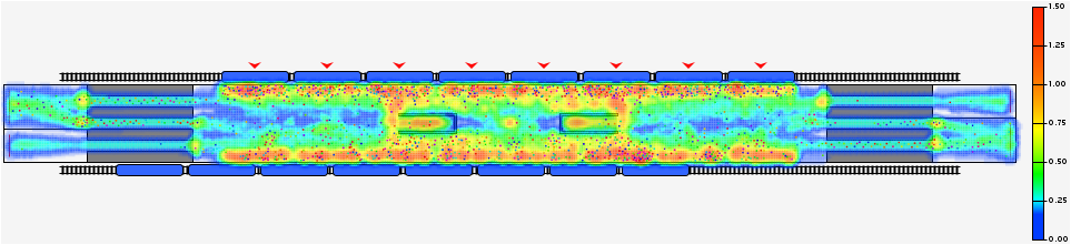
The red color indicates the critical density (by default it is equal to 1.5 units/m²). The blue color is used for low densities. If the density in some area is zero, the density map for that area is not drawn at all.

For example, the legend shown in the figure above tells us that the yellow color on the map corresponds to a density of 0.75 pedestrians/m².

You can change the logarithmic color scheme to linear or some other scheme, turn attenuation on or off, and so on.

To add a density map

1. Drag the  Density Map element into the graphical editor from either section of the Space Markup palette:  Material Handling or  Pedestrian. At the runtime it will show the density map legend. The legend displays the correspondence between density values and colors on the density map.

   

2. In the properties, specify the Type of the density map:
   • Pedestrian — to display the density map for pedestrians.
   • Transporter — to display the density map for transporters with free space navigation.
3. You can select your density map to display either historical data, that is, values collected from the start of the model run (the Complete model run option of the Time period parameter) or values collected over the specified period of time (the Sliding window option of the Time period parameter). You can also select the Displayed density value: either Maximum or Mean.
   The amount of memory required to process the data increases proportionally to the size of the sliding window.
4. If you are collecting maximum density values over an entire model run, these values can be displayed either as maximum observed density values (if attenuation is turned off) or as the actual density map for the most recent period of time (if attenuation is turned on). With attenuation turned on, as the density decreases, the color for the corresponding zone on the density map will change accordingly, but not immediately. To turn the attenuation on, select the Enable attenuation check box.
5. If you are unhappy with the way the density map is painted over the layout, making it hard to see, you can increase the transparency of the density map using the Transparency slider.
6. The density map is often used to identify areas of critical density. At model runtime, the areas with density values equal to or greater than the critical density threshold are colored in red (unless some other colors are set using the Custom option of the Color scheme property). By default, the critical density value is 1.5 units/m². Units here are either pedestrians or transporters, depending on the type of density map. You can change this value in the Critical Density parameter.
7. By default, AnyLogic uses a logarithmic color scheme. In this case the color changes logarithmically from the “minimum” color (blue) to the “maximum” color (red). This color scheme is often used when you need to pay attention only to the density values close to the critical value threshold. You can change the logarithmic color scheme to the linear scheme by selecting the Linear option of the parameter Color scheme. This is the simplest color scheme: the color changes linearly from the “minimum” color to the “maximum” (red) color. You can even define your own color scheme by selecting the Custom option of the Color scheme property.

General

Name — The name of the shape. The name is used to identify and access the shape.

Ignore — If selected, the shape is excluded from the model.

Visible on upper agent — If selected, the shape is also visible on the upper agent where this agent lives.

Lock — If selected, the shape is locked. Locked shapes do not react to mouse clicks — it is impossible to select them in the graphical editor until you unlock them.

Visible — Here you specify whether the density map legend is visible on the animation at the model runtime, or not. Using the control, choose yes or no.

Type — Specifies the type of agent for which the density map will be displayed: either Pedestrian or Transporter.

Time period — Specifies how density data is collected. The default option is Complete model run, where data is collected from the start of the model run to the present. The other option is Sliding window, which represents a length of time over which the density data is collected. For example, if you specify the sliding window of 5 minutes, the density map will display only the information collected over the last 5 minutes, ignoring any earlier data.

Sliding window — [Visible if Time period: Sliding window] Specifies the exact time period over which the data is collected.

Displayed density value — Specifies which density value will be used to display on the density map. It can be either Maximum value or Mean value.

Enable attenuation — If selected, the density map will be shown with attenuation. In this case, the actual density map for the most recent period of time will be shown, not the maximum observed densities. When the density goes down, the color for the corresponding zone on the density map changes accordingly (but not immediately, with the specified delay).

Transparency — Specifies the transparency level for the density map. Use the slider to select a value in the range [0..100%]. 100% means fully transparent map (the density map is not visible), 0% means fully opaque density map (the animation below the density map is not visible at all).

Critical density — Specifies the critical density value. All areas with densities equal to or greater than the critical density threshold will be painted red in the animation (unless some other color is set with Custom as the Color scheme).

Color scheme — The color scheme for the density map. There are three options available:

• Logarithmic — The color will change logarithmically from the “minimum” color (blue) to the “maximum” color (red). This color scheme is often used when you need to pay attention only to the density values close to the critical value threshold.
• Linear — The simplest color scheme: color will change linearly from the “minimum” color (blue) to the “maximum” color (red).
• Custom — You can define your own color scheme and define the correspondence between colors and density values in the Custom color field below.

Custom color — [Visible if Color scheme: Custom] If you want to define a custom color scheme for the density map, specify the expression that will return different colors depending on the density value (you can obtain the density value using the local variable density).

You can see an example of such an expression set up as the default value:

density > self.criticalDensity * 0.7 ? red : transparent

It defines that the color red will be used for the densities that are higher than the specified threshold value (70% of the critical density value). For the lower densities, the density map will not be drawn at all.

If the transparency argument specified in your custom code equals 0, i.e. the color that your code returns is fully opaque, then the setting of the Transparency parameter will be applied to your custom color scheme.

Position and size

Level — The name of the level for which the density map will be displayed.

X — The X-coordinate of the density map legend.

Y — The Y-coordinate of the density map legend.

Width — The width of the density map legend (in pixels).

Height — The height of the density map legend (in pixels).

Advanced

Show in — The option defines whether you want the density map to be shown both In 2D and 3D animation, or in 2D only, or in 3D only. Since density map can be shown only in 2D animation, the 2D only option is selected and the control is disabled.

Show name — If selected, the shape’s name is displayed on a presentation diagram.

Type

Function	Description
DensityMapType getType()	Returns the type of the density map depending on whom the statistics are collected: either pedestrians or transporters. Valid values: PEDESTRIAN_MAP_TYPE — the density map is displayed for pedestrians TRANSPORTER_MAP_TYPE — the density map is displayed for transporters

Displayed density value

Function	Description
DensityMapDisplayedValue getDensityValue()	Returns the type of value used to build the density map. Possible values: DENSITY_VALUE_MAX — maximum density value DENSITY_VALUE_MEAN — mean density value
void setDensityValue(DensityMapDisplayedValue valueType)	Sets the type of density value used to build the density map. valueType — a constant defining density value type. Possible values: DENSITY_VALUE_MAX — maximum density value DENSITY_VALUE_MEAN — mean density value

Statistics

Function	Description
double currentDensity(double x, double y)	Returns the current density value in the area neighboring the specified point, units/m2. The units here mean either pedestrians or transporters, depending on the density map type. This value does not reflect exactly the current situation, it accumulates historic data. x — X-coordinate of the point y — Y-coordinate of the point
double maximumDensity(double x, double y)	Returns the maximum density value in the specified point, units/m2. x — X-coordinate of the point y — Y-coordinate of the point
void reset()	Resets the values of the density map that the user can see and obtain by calling the maximumDensity() function to the current values of density.

Color scheme

Function	Description
DensityMapColorScheme getColorScheme()	Returns the color scheme of the density map. Valid values: LINEAR_COLOR_SCHEME LOGARITHMIC_COLOR_SCHEME CUSTOM_COLOR_SCHEME
void setColorScheme(DensityMapColorScheme colorScheme)	Sets the new color scheme. colorScheme — the new color scheme. Valid values: LINEAR_COLOR_SCHEME LOGARITHMIC_COLOR_SCHEME CUSTOM_COLOR_SCHEME
double getCriticalDensity()	Returns the critical density for the density map, in units/m2.
void setCriticalDensity(double criticalDensity)	Sets the new critical density for the density map, in units/m2. criticalDensity — the new critical density value

Attenuation and transparency

Function	Description
double getTransparency()	Returns the density map transparency. The value is in the range [0, 1], 0 means fully opaque, 1 means fully transparent.
void setTransparency(double transparency)	Sets the new density map transparency. transparency — the new transparency value. The value should be in the range [0, 1], 0 means fully opaque, 1 means fully transparent.
boolean isEnableAttenuation()	Returns true if the density map is shown with attenuation; returns false otherwise.
void setEnableAttenuation(boolean enable)	Turns density map attenuation on/off. enable — attenuation. If enable is true — the density map is shown with attenuation, if it is false — attenuation is turned off.

Visibility

Function	Description
void show()	Shows the density map.
void hide()	Hides the density map.
void display(boolean flag)	Sets the visibility of the density map. flag — visibility. If flag is true — the density map is displayed. If it is false — the density map is invisible.
boolean isVisible()	Returns true if the density map legend is visible; returns false otherwise.
void setVisible(boolean v)	Sets the visibility of the density map legend. v — visibility. If v is true — the density map legend is set to be visible, if it is false — not visible.

Level

Function	Description
Level getLevel()	Returns the level, for which the density map is displayed.

Legend position

Function	Description
double getX()	Returns the X-coordinate of the density map legend.
double getY()	Returns the Y-coordinate of the density map legend.
void setX(double x)	Sets the X-coordinate of the density map legend. x — new X-coordinate
void setY(double y)	Sets the Y-coordinate of the density map legend. y — new Y-coordinate

Legend size

Function	Description
double getWidth()	Returns the width of the density map legend (in pixels).
double getHeight()	Returns the height of the density map legend (in pixels).
void setWidth(double width)	Sets the width of the density map legend (in pixels). width — the new width
void setHeight(double height)	Sets the height of the density map legend (in pixels). height — the new height

Removal

Function	Description
void remove()	Removes the density map from the presentation. If the map is not a part of presentation, the function does nothing. Removal from the presentation does not necessarily mean removing from the model logic, since logical networks and routes may have been created before the removal and survive it.

How can we improve this article?

Send